Adaptive Attention

This is a technical blog post for a novel, end-to-end, adaptive attention architecture. Slides can be found here.

Background and Motivation

Throughout the last decade, two distinct types of machine learning architectures have emerged: transformers and linear attention variants, which include RNNs, SSMs, test-time learners, and more. These two architectures occupy opposite ends of a spectrum. Transformers are extrapolators, storing every new token into a growing KV cache, whereas linear attention models are interpolators, compressing each token of information as an update to the same fixed weights.

Transformers are expressive but expensive to run training and inference at long contexts, since each new query must attend to all past keys and values. This means that purely transformer-based models waste lots of compute on tasks like multimodal generation and needle in a haystack, where most tokens are redundant and intelligent selection would greatly save FLOPs. Transformers also need tokenization to succeed, which is human-designed, clunky, and not end-to-end. Finally, approaches to KV cache compression, such as quantization and eviction are often heuristics-based, not parallelizable during pre-training, or inexpressive.

In contrast, linear attention models are efficient, only requiring linear-time generation. Transformers function like databases, where each new observation is appended to a KV cache, whereas linear models function like brains, whose fixed parameter counts continually update. However, such models only have a fixed state to store progressively increasing context, which hurts precise recall abilities. Also, all linear attention variants make assumptions on how to organized the state matrix. For example, MesaNet attempts to solve the global retrieval regression $\mathcal{L}(M_{n}) = \sum _{i=1} ^{n} \alpha_i \lVert M_{n}k_{i} - v_{i} \rVert^2$, DeltaNet solves a local retrieval regression $\mathcal{L}(M_{n}) = \lVert M_{n}k_{n} - v_{n} \rVert^2$, and Log-Linear attention assumes a logarithmic compression schedule.

H-Net (Hwang, Wang, Gu, 2025)) attempts to solve these problems through dynamic chunking, where the model learns a chunking scheme that attempts to approach a set compression ratio by predicting chunk boundaries. However, chunking is greedy, only considering differences between consecutive tokens, which both doesn't consider accumulating differences across sequence ranges and isn’t as expressive, particularly for multimodal use cases like video generation. Finally, the compression ratio is fixed: ideally we'd want the model to learn when it's useful to keep vs. compress tokens.

So, the two main questions we aim to answer are:

1. How can we teach the model to dynamically select how much compute it wants to use for attention? Transformers and linear attention models only perform $O(n)$ and $O(1)$ next-token prediction, respectively, but depending on the task necessity, ideally we can express $O(\log n)$ or $O(\sqrt{n})$ or some other variant with the same dense model.
2. How can we effectively compress in a maximally expressive way? There are a plethora of linear attention variants with different update rules and different tradeoffs: can we create an architecture that can express all of these variants?

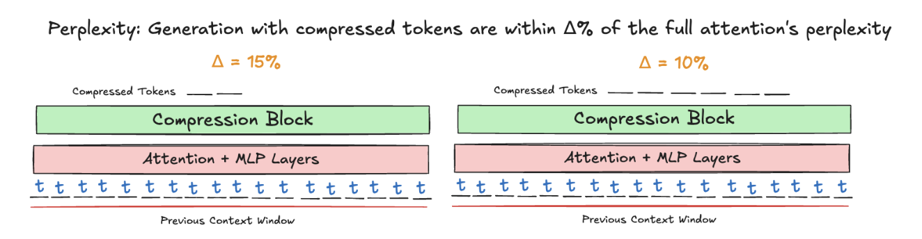
This is the heart of my new adaptive attention model, which compresses inputs in the sequence dimension. The compression ratio is computed by a learned module that predicts how much compression would impact the task performance. We measure this by using the difference of the perplexity of the model when using the compressed tokens with respect to the model's full-attention perplexity.

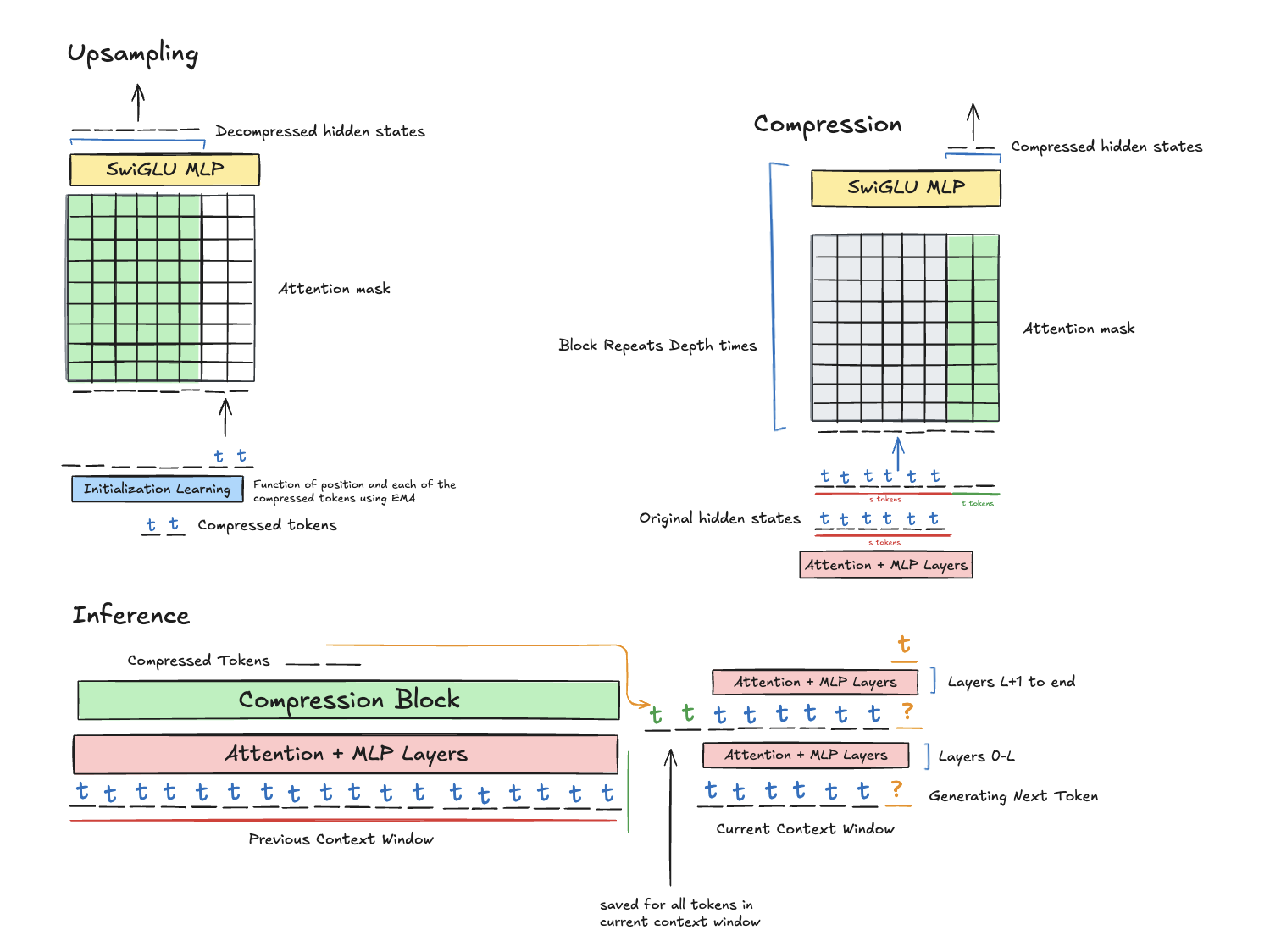
Compression

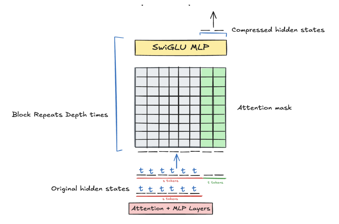
We insert our compression layer between two transformer blocks, where it shrinks the sequence dimension from [b, s, d] to [b, t, d] where t < s. We use a suffix initialization scheme to initialize $t$ new tokens, which attend to all of the original $s$ tokens (which are frozen during attention to save compute). This attention matrix is $O(nt),$ which lets us express any time complexity between linear and full attention, depending on whether $t$ is $O(1), O(n),$ or something else. Since the matrix is dense, it can theoretically express Mamba-2, DeltaNet, and all similar state matrix architectures, since all of these architectures have semi-separable matrices in their parallel forms. We combine attention and SwiGLU MLP blocks to maximize retrieval ability, since according to Hopfield theory, attention has a theoretically exponential memorization capacity.

Parallelization

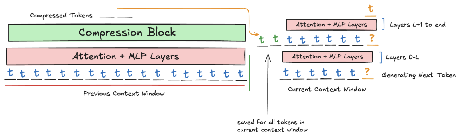
Greedy, per-step compression strategies wouldn't work because pre-training wouldn't be parallelizable. Instead, we select an amortized strategy, where a separate module runs parallel to the main module during inference and compresses the KV cache in an online format. This is similar to most "append persistent KV" approaches, such as in Titans (Behrouz, 2024), except it is more efficient since it runs parallel to generation, and it is more general than Titans' approach of compressing once per context window.

Pre-Training

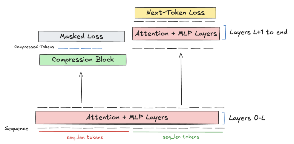
Now, we can make the amortized approach work for pre-training. Before we build up to the adaptive compression scheme, we first fix our compression ratio and the number of tokens we will compress - note that our compression block is inherently flexible to multiple compression ratios and token counts, as attention is applied independently and the SwiGLU MLP transforms in the feature dimension.

So, we fix seq_len original tokens, which represents the past context window that we prepare to compress. We pass this through the first $L$ transformer blocks, where an attention mask ensures that the first seq_len tokens can only causally see each other, and the last seq_len tokens cannot peek at any of the first seq_len tokens. This mimics inference, since the first layers of the model cannot peek at the previous context window. Then, at layer $L$, the prefix of length seq_len is compressed into a smaller number of tokens, say $t$. These hidden states are prepended to the sequence's hidden states. The combined set of hidden states are then passed through the rest of the model with standard causal attention on the $s+t$ hidden states throughout. By masking the loss on the original compressed tokens, we ensure that the model only is incentivized to perform continual learning, and learns representations for the compression layer that align with setting up the model for successful continual learning.

For evaluations, we pre-train on Project Gutenberg texts, since the primary benefit of the added compressed hidden states is to provide more useful information for in-context learning, and we need the documents to be long enough such that the seq_len prefix tokens are part of the same text as the seq_len suffix tokens, and thus provide meaningful information. This setup also allows us to run numerous architectural ablations, such as hyperparameter choice, choice of compressed token initialization, etc.

Multiple Compression Ratios

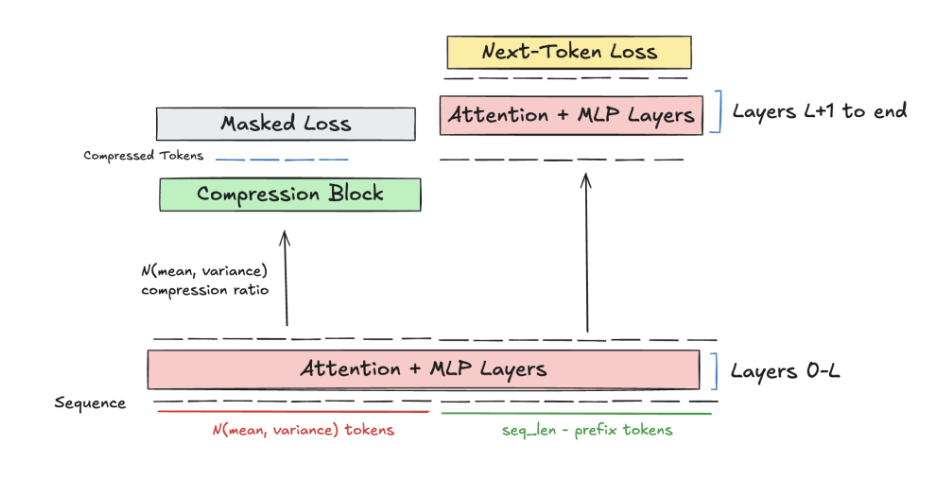
When we introduce our module that adaptively predicts our compression ratio, we want our compression module to generalize to variable prefix tokens and compression ratios. We do this by randomly sampling the prefix and compression ratio for each batch from a uniform distribution with growing variance throughout training.

Recursive Compression

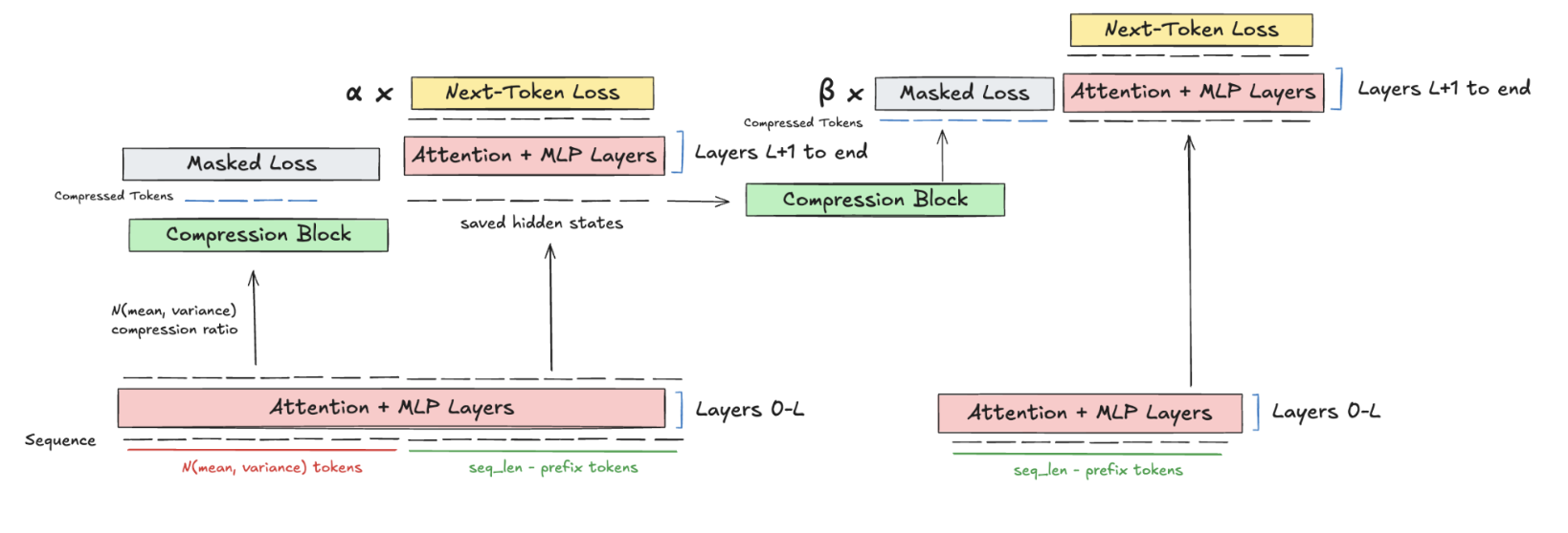
One issue is that during continual learning, as we continually compress, we will have hidden states that have been compressed multiple times, and we want to learn meaningful representations for such hidden states. We do this by recurrently caching the compression prefix and new hidden states at each iteration.

Learning the Adaptive Loss Function

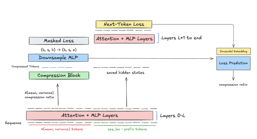
We want to incorporate a loss function that incentivizes the model to compress only when it would greatly benefit the model. We do this by curating a diverse set of prompts $x$ and curating the difference in NLL loss $\Delta = \text{Loss(Compressed)} - \text{Loss(Full)}$ over a diverse set of compression ratios. Then, we train a separate module that uses a down-projecting MLP to convert the shrunken hidden state sequence into a set of low-dimensional latents, and a sinusoidal embedding of the loss difference $\Delta$ to predict the compression ratio $\frac{p}{\text{seq\_len}}.$ Then, we manually set some threshold $\Delta^*$, our error tolerance with respect to full attention, and estimate the compression ratio needed. Under this scheme, the model predicts a significant compression ratio on trivial tasks and random noise, whereas the model chooses to use more attention on summarization tasks.

Evaluations

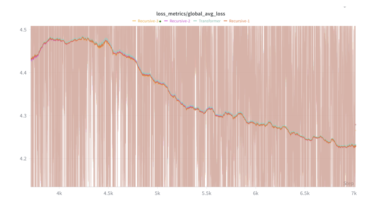
We evaluate the training perplexity on Project Gutenberg when simulating a baseline transformer with num_compressed_tokens tokens prepended to the hidden states after layer $L$ for FLOP matching. We compare this with our adaptive attention module after $1, 2,$ and $3$ compressions, which is equivalent to how far our context length has been extended, and observe that performance with respect to baseline increasing as context length grows, highlighting our architecture's promising ability to improve continual learning. We also plan on evaluating our model on long-context benchmarks like LongBench v2, Loong, LV‑Eval, L‑Eval, and BAMBOO.

Applications

• Data processing. Database queries will tremendously benefit from adaptive attention, since some queries might attend to many rows of the database, whilst others won't need much attention at all.
• Video generation. Adaptive attention greatly improves attention efficiency and resolves multimodal tokenization challenges with respect to spatial and temporal locality that make video generation difficult.

Future Directions

• Vincent Hermann et. al. (2025) proposes a PHi layer that uses an autoencoder layer to predict the difficulty of a task. For a wide sample of tasks, we can measure the compression ratio predicted by our module and evaluate its correlation with the PHi loss.

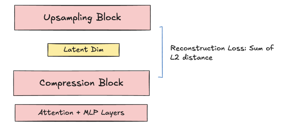
• We measure, given a fixed compute and parameter budget, the reconstruction loss we can attain by pre-training the compression block and the upsampling block from scratch, as a baseline (the transformer layers are frozen). We compare this with the reconstruction loss after importing and freezing the compression block to determine how optimized the learned compression block for next-token prediction is for memory. If the reconstruction losses are close, then our learned compression block through next-token prediction generally remembers most of the possible information that the block can store.

• Interpretability: We pre-train the model on the CLEVR dataset, which consists of simple object identification tasks. We use one compression token for the image, in an image with 3 items, to determine if it focuses attention on the items.

• Tokenization: We import the compression before the first transformer layer, and benchmark the ability of our layer to perform compression with respect to standard tokenization (with tokens matched) to understand our layer’s potential for tokenization.

We thank Lambda Labs as a compute partner, and Han Guo, Jyo Pari, and Shivam Duggal for valuable insights and perspectives that have helped shape the model and blog post. An earlier version of this architecture can be found here.